My 2018 Year in Gaming
Introduction
Starting back in 2017, I started recording my time spent gaming each day and which game. This will be a brief breakdown of time spent gaming using R and packages dplyr, ggplot2, and directlabels. Using dplyr for data manipulation, ggplot2 and directlabels for plotting.
Game Time
We have already loaded the data, so lets start taking a look.
dat.sum <- dat %>% group_by(Game) %>% summarise(tot.time.minutes=sum(Time..minutes.)) %>% arrange(desc(tot.time.minutes))

ggplot(dat.sum, aes(Game, tot.time.minutes)) + geom_col() + theme(axis.text.x = element_text(angle = 90, hjust = 1, vjust=0.5)) + ylab("2018 Total Time (minutes)") + xlab("")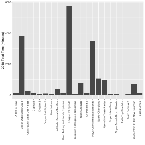
knitr::kable(dat.sum, align="c")| Game | tot.time.minutes |
|---|---|
| League of Legends | 5756 |
| Call of Duty: Black Ops 4 | 3835 |
| PlayerUnknown’s Battlegrounds | 3494 |
| Quake Champions | 1070 |
| Rise of the Tomb Raider | 986 |
| Nier: Automata | 774 |
| Wolfenstein II: The New Colossus | 722 |
| Hellblade: Senua’s Sacrifice | 388 |
| Call of Duty: Black Ops 4 beta | 235 |
| Cuphead | 142 |
| Keep Talking and Nobdy Explodes | 140 |
| A Hat In Time | 117 |
| Overcooked 2 | 115 |
| Yooka Laylee | 110 |
| Dragon Ball FighterZ | 97 |
| Team Fortress 2 | 64 |
| Super Mario Party | 62 |
| Lovers in a Dangerous Spacetime | 59 |
| Super Smash Bros. Ultimate | 43 |
| Hearthstone | 39 |
| Destiny 2 | 34 |
| TableTop Simulator | 11 |
Games like League of Legends, Call of Duty: Black Ops 4, and PlayerUnknown’s Battlegrounds stand out as games played the most. This is entirely due to the multiplayer aspect. Other games, like Team Fortress 2 and Hearthstone I played a lot in 2017 and earlier but have since stopped playing. The Switch games, I only recently started playing at end of the year, so very low. The same is for TableTop Simulator.
Removing the low played, say less than 3 hours, we will plot up the cumulative time played through the year.
dat.filt <- dat[dat$Game %in% dat.sum$Game[dat.sum$tot.time.minutes >= 180],]
# Get cumulative sum
dat.cumsum <- dat.filt %>% group_by(Game) %>% mutate(cv=cumsum(Time..minutes.))

ggplot(dat.cumsum, aes(x=Date, y=cv, colour=factor(Game))) +
  geom_line(size=1) +
  geom_point() +
  geom_dl(aes(label=Game), method=list(dl.trans(x=x-0.5,y=y+0.2), "last.points", cex=0.8)) +
  scale_colour_discrete(guide='none') +
  ggtitle("2018 Cumulative Gaming Time") +
  ylab("Cumulative Game Time (Minutes)")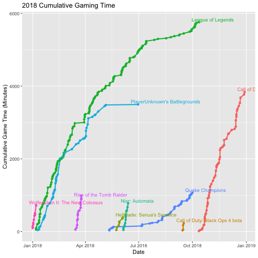
From this, even though League of Legends has my highest play time from 2018, I stopped playing around October and Call of Duty: Black Ops 4 takes over.
Looking back at total time played, lets take a look at my monthly gaming time.
# Total game time per month
monthly.sum <- dat %>% mutate(month=format(Date, "%m")) %>% group_by(month) %>% summarise(total.minutes=sum(Time..minutes.))
ggplot(monthly.sum, aes(month,total.minutes)) +
  geom_col() +
  ggtitle("Month vs Gaming Time (minutes)") +
  xlab("Month") +
  ylab("Total Gaming Time (minutes)")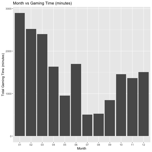
Winter months here are cold, mostly relating to the time played being higher. I also know that July, August, and September I had spent almost all my free time cycling, running, or just being outside while it was nice. The month of June is larger as I had my wisdom teeth out during this time and could not get out as much during the healing.
Lets take a look at the monthly time based on game:
monthly.game <- dat %>%
  mutate(month=format(Date, "%m")) %>%
  group_by(month, Game) %>%
  summarise(total.minutes=sum(Time..minutes.)) %>%
  arrange(month, desc(total.minutes), Game)
knitr::kable(monthly.game, align="c")| month | Game | total.minutes |
|---|---|---|
| 01 | League of Legends | 1233 |
| 01 | PlayerUnknown’s Battlegrounds | 776 |
| 01 | Wolfenstein II: The New Colossus | 722 |
| 01 | Cuphead | 142 |
| 01 | Hearthstone | 22 |
| 02 | PlayerUnknown’s Battlegrounds | 1394 |
| 02 | League of Legends | 1014 |
| 02 | Dragon Ball FighterZ | 97 |
| 02 | Hearthstone | 17 |
| 03 | Rise of the Tomb Raider | 986 |
| 03 | League of Legends | 958 |
| 03 | PlayerUnknown’s Battlegrounds | 408 |
| 03 | Team Fortress 2 | 48 |
| 04 | PlayerUnknown’s Battlegrounds | 723 |
| 04 | League of Legends | 695 |
| 04 | Keep Talking and Nobdy Explodes | 140 |
| 04 | Lovers in a Dangerous Spacetime | 59 |
| 04 | Team Fortress 2 | 16 |
| 05 | League of Legends | 370 |
| 05 | Hellblade: Senua’s Sacrifice | 274 |
| 05 | PlayerUnknown’s Battlegrounds | 179 |
| 05 | Quake Champions | 129 |
| 06 | Nier: Automata | 774 |
| 06 | League of Legends | 684 |
| 06 | Hellblade: Senua’s Sacrifice | 114 |
| 06 | Yooka Laylee | 110 |
| 06 | PlayerUnknown’s Battlegrounds | 14 |
| 07 | League of Legends | 316 |
| 07 | Quake Champions | 110 |
| 07 | A Hat In Time | 76 |
| 08 | Quake Champions | 422 |
| 08 | League of Legends | 102 |
| 09 | Quake Champions | 382 |
| 09 | Call of Duty: Black Ops 4 beta | 235 |
| 09 | League of Legends | 190 |
| 09 | A Hat In Time | 41 |
| 10 | Call of Duty: Black Ops 4 | 1235 |
| 10 | League of Legends | 194 |
| 10 | Quake Champions | 27 |
| 11 | Call of Duty: Black Ops 4 | 1316 |
| 11 | Destiny 2 | 34 |
| 11 | TableTop Simulator | 11 |
| 12 | Call of Duty: Black Ops 4 | 1284 |
| 12 | Overcooked 2 | 115 |
| 12 | Super Mario Party | 62 |
| 12 | Super Smash Bros. Ultimate | 43 |
One last thing, looking at the day of the total playtime for each day of the week:
daily.sum <- dat %>%
  group_by(weekdays(Date)) %>%
  summarise(tot.time.minutes=sum(Time..minutes.))
daily.sum$`weekdays(Date)` <- factor(daily.sum$`weekdays(Date)`, ordered=T, levels=c("Monday", "Tuesday", "Wednesday", "Thursday", "Friday", "Saturday", "Sunday"))
daily.sum <- daily.sum[order(daily.sum$`weekdays(Date)`),]
names(daily.sum) <- c("Weekday", "Total.Time.Minutes")
knitr::kable(daily.sum, align="c")| Weekday | Total.Time.Minutes |
|---|---|
| Monday | 1982 |
| Tuesday | 1533 |
| Wednesday | 1548 |
| Thursday | 995 |
| Friday | 4277 |
| Saturday | 5164 |
| Sunday | 2794 |